Object recognition is a crucial technology in the field of computer vision and artificial intelligence, enabling machines to identify and classify various objects within digital images or video feeds. By mimicking the human ability to recognize and categorize objects, object recognition has paved the way for advancements across industries, from autonomous driving and facial recognition to medical imaging and industrial automation. With recent strides in machine learning and deep learning, particularly with convolutional neural networks (CNNs), the accuracy and efficiency of object recognition systems have dramatically improved.
Patterns and Pattern Classes

In pattern recognition, understanding “patterns” and “pattern classes” is fundamental. Here’s a structured breakdown of the mathematical concepts and examples discussed.
1. Patterns and Pattern Classes
- Pattern: An arrangement of descriptors (or features) used to represent an object or entity.
- Descriptor: An attribute or characteristic of an object, often called a “feature” in pattern recognition literature.
- Pattern Class: A family of patterns sharing common properties. Each pattern class is denoted by , where represents the class number.
In machine-based pattern recognition, the goal is to assign patterns to their respective classes with minimal human intervention. This involves various techniques and mathematical tools.
2. Common Pattern Arrangements
Three common forms of patterns are vectors, strings, and trees, each suited to different types of descriptions:
a. Pattern Vectors (Quantitative Descriptions)
Represented by bold lowercase letters (e.g., x, y, z), pattern vectors are used for quantitative features.
A pattern vector is a column matrix:
where each is a descriptor, and is the total number of descriptors. This vector is also expressed as:
where denotes transposition.
Example: Iris Classification (Fisher, 1936)
Each iris flower is described by two measurements: petal length and width, forming a 2D pattern vector:
Here, is petal length, and is petal width. The pattern classes, , , and , represent the varieties “setosa,” “virginica,” and “versicolor,” respectively.
By plotting these vectors in a 2D Euclidean space, each flower is represented as a point, allowing us to distinguish classes based on the separation of points.
b. Pattern Vectors in Higher Dimensions
In some cases, descriptors are sampled at specific intervals, creating high-dimensional vectors. For example:
Here, each represents a sampled point, and is the amplitude at that point. These vectors form points in an -dimensional Euclidean space, where patterns are visualized as “clouds” in the space.
c. Structural Descriptions (Strings and Trees)
For certain applications, structural descriptions are more effective than quantitative measures.
i. String Descriptions
Patterns with repeated structures can be represented as strings. For example, a staircase pattern may consist of alternating primitive elements, such as “A” and “B”. A staircase can then be represented by the string:
The order of these elements captures the pattern structure.
ii. Tree Descriptions
Tree structures represent hierarchical relationships, as seen in spatial and image analysis. For example, in a satellite image of a city, we could use the following hierarchy:
- Root node: Entire image
- Next level: Distinguishes “downtown” and “residential areas”
- Further levels: Separate “housing,” “highways,” and “shopping malls” within residential areas
This hierarchical representation allows for detailed structural analysis.
3. Pattern Recognition Techniques
Selecting descriptors impacts the success of pattern recognition. Examples include:
- Quantitative Techniques: These use measurements to create pattern vectors, as seen in iris classification.
- Structural Techniques: These analyze spatial relationships, like fingerprint minutiae (e.g., ridge endings and branch points), which are used in fingerprint recognition.
Example Problem: Recognition of Shapes with Noise
Suppose we want to classify noisy shapes, each represented by a 1D signature. By sampling the signature at intervals, we obtain a pattern vector in -dimensional space. Alternatively, we could compute statistical features, such as moments, for each signature and use these in our pattern vector.
Recognition Based on Decision-Theoretic Methods
Recognition based on decision-theoretic methods is a fundamental approach in pattern recognition that leverages statistical probability and optimization techniques to classify patterns. These methods rely on decision functions that use feature vectors, distances, and probability distributions to assign patterns to classes, with a primary goal of minimizing misclassification errors.
Here, we expand on the mathematical concepts behind these methods, including the Minimum Distance Classifier, the Bayes Classifier, and Correlation-Based Matching, along with examples that illustrate these principles in action.
1. Decision-Theoretic Framework
In decision-theoretic pattern recognition, we use decision functions for each class , where is an -dimensional feature vector. A pattern is assigned to the class with the highest value of , that is:
The set of points where forms the decision boundary separating class from . Decision boundaries play a critical role in defining the regions of the feature space assigned to each class.
2. Minimum Distance Classifier
The Minimum Distance Classifier is a straightforward classifier that assigns a pattern vector to the class whose prototype vector (often the mean vector) is closest to in terms of Euclidean distance. This method assumes that each class can be represented by a prototype or mean vector defined as:
where is the number of training samples in class .
Euclidean Distance Calculation
For a new pattern , we compute the Euclidean distance from to each class prototype as:
where denotes the -th component of the mean vector .
Classification Rule
The pattern is assigned to the class with the smallest :
Example: Suppose we classify two types of iris flowers based on petal length and width. The mean vectors for each class are calculated, and the classifier computes the Euclidean distance between a new flower’s feature vector and each class mean. The class with the smallest distance is chosen as the classification for the new flower.
3. Bayes Classifier
The Bayes Classifier is an optimal statistical classifier that minimizes the average probability of misclassification by assigning patterns based on posterior probabilities. The Bayes classifier uses Bayes’ theorem to compute the posterior probability , the probability of belonging to class given the observed data.
Bayes Decision Rule
A pattern is assigned to the class if:
Using Bayes’ theorem, the posterior probability can be rewritten as:
where:
- : Likelihood of observing given that it belongs to class .
- : Prior probability of class .
- : Marginal probability of observing across all classes, acting as a normalizing constant.
The decision rule simplifies to:
Zero-One Loss Function
A common choice in Bayes classification is the 0-1 loss function, where the loss is 0 for correct classifications and 1 for incorrect ones. The Bayes classifier then minimizes the probability of misclassification by assigning to the class with the highest posterior probability.
Gaussian Bayes Classifier
If the probability densities follow a multivariate Gaussian distribution, the likelihood of given class with mean vector and covariance matrix is:
where is the determinant of .
The Bayes decision function for each class then becomes:
The classifier assigns to the class with the highest .
Example: In remote sensing, multispectral data from different spectral bands can be used to classify land cover types. Each pixel is represented as a vector, and the Bayes classifier assigns each pixel to a land cover class based on estimated Gaussian densities for each class.
4. Correlation-Based Matching
Correlation-based matching is used when patterns are matched with predefined templates, especially in applications involving images or shapes. This method compares patterns based on similarity rather than probability, using a correlation coefficient as a measure of similarity.
Normalized Correlation Coefficient
The normalized correlation coefficient between a pattern and a template is given by:
where and are the mean values of and , respectively. This coefficient ranges from -1 to 1:
- indicates a perfect positive correlation.
- indicates a perfect negative correlation.
- indicates no correlation.
Template Matching Rule
Assign to the class represented by template if is maximized for that template among all others:
Example: In satellite image processing, a correlation-based matcher can identify a specific feature within an image (such as the eye of a hurricane) by finding the region with the highest correlation with a template of the feature.
Practical Applications of Decision-Theoretic Methods
Example 1: Character Recognition Using Minimum Distance Classifier In automated reading of bank checks, characters are represented by feature vectors based on pixel densities or boundary points. The minimum distance classifier compares a new character’s vector with prototype vectors of each character, assigning it to the class with the smallest distance.
Example 2: Land Cover Classification Using Bayes Classifier In remote sensing, each pixel of a multispectral image is classified as water, urban, or vegetation using the Bayes classifier. This classifier uses prior knowledge of land cover probabilities and multispectral data from sample regions to compute mean vectors and covariance matrices for each class.
Decision-theoretic methods provide a robust framework for pattern recognition, using probabilistic and mathematical criteria to minimize misclassification risks. The choice of a method depends on the nature of the data, the degree of overlap between classes, and the computational requirements of the application.
Structural Methods


In pattern recognition, structural methods leverage the structural relationships of a pattern’s shape rather than relying solely on numerical representations. Unlike quantitative approaches, structural techniques consider the inherent structure of patterns, making them particularly effective for boundary shape recognition. A commonly used method within structural pattern recognition involves string representations of shapes, which enables the classification of complex shapes through symbolic descriptions.
In this discussion, we cover two structural methods for boundary shape recognition based on string representations: Matching Shape Numbers and String Matching.
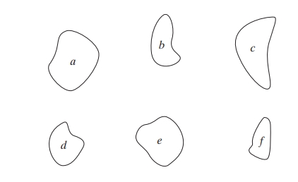
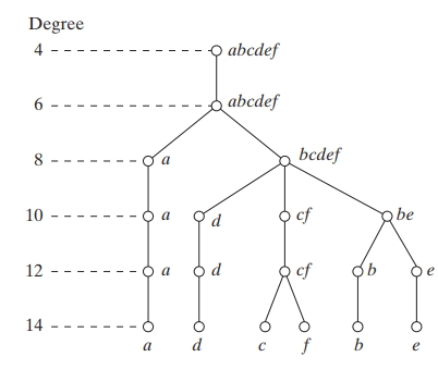
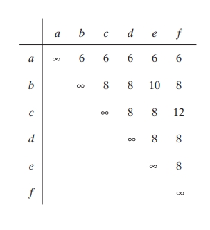
Matching Shape Numbers
In many cases, shapes can be represented by numbers based on their boundaries, known as shape numbers. This method is similar to the minimum distance concept introduced for pattern vectors, but here, it applies specifically to the comparison of boundaries using shape numbers. The idea is to compare shapes based on how similar their boundary representations are.
Shape Representation with Shape Numbers: A shape number provides a numerical description of a closed boundary, often encoded using a 4-directional chain code. Each segment of the boundary is assigned a numerical value depending on its direction relative to the previous segment. For example, a rightward movement might be coded as
0, an upward movement as1, a leftward movement as2, and a downward movement as3.Defining Similarity (Degree of Similarity): The degree of similarity between two shapes and can be determined by comparing their shape numbers at successive orders, as long as they coincide. If and denote the shape numbers of shapes and at the -th order, they are considered similar up to order if:
In this case, the degree of similarity is the largest value of for which the shape numbers coincide.
Defining Distance (Dissimilarity Measure): The distance between two shapes and is the inverse of their degree of similarity:
This distance measure satisfies several properties:
- Non-negativity:
- Identity of Indiscernibles: if and only if
- Symmetry:
Example: Suppose we have two shapes, each represented by a 4-directional chain code sequence. Let’s say their shape numbers coincide up to the 6th order. In this case, the degree of similarity , and thus, the distance . If another pair of shapes only matches up to the 4th order, their distance will be , indicating that they are less similar than the previous pair.
A larger degree of similarity (higher ) implies that the shapes are more alike, whereas a larger distance suggests that they are less similar.
String Matching
String matching is another approach used for comparing shapes based on boundary representations encoded as strings. This method allows for matching and alignment of boundaries represented as strings, where each boundary point is translated into a symbol, creating a sequential symbolic representation of the boundary.
String Representation: Suppose we have two region boundaries, and , represented by strings and . A boundary is encoded into a string by assigning each boundary segment a symbol (such as a chain code), resulting in strings that can be compared symbol by symbol.
Counting Matches and Mismatches: Let be the number of matching symbols between and , where a match occurs if the symbols at a given position in both strings are the same. The number of mismatches can be defined as:
where and denote the lengths of the strings and . If , then , which implies that the two strings are identical.
Similarity Measure (Ratio of Matches): A similarity measure between the two strings can be defined as:
where approaches 1 for a perfect match and 0 if there are no matching symbols. This measure is maximized by aligning the strings optimally to maximize .
Example: Suppose we compare two strings, and , with the same length (4). Comparing the symbols at each position, we find that three positions match. Therefore, and:
indicating a high degree of similarity between the two shapes.
Normalization and Optimal Alignment: To achieve the best comparison, it may be necessary to shift one of the strings circularly (wrapping around the end) and calculate for each shift. The highest value of across all shifts indicates the best alignment and the closest match between the two strings.
References
- Duda, R. O., Hart, P. E., & Stork, D. G. (2001). Pattern Classification. John Wiley & Sons.
- Goodfellow, I., Bengio, Y., & Courville, A. (2016). Deep Learning. MIT Press.
- Bishop, C. M. (2006). Pattern Recognition and Machine Learning. Springer.
