Image Segmentation

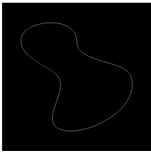
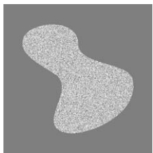
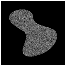
Image segmentation is the process of partitioning an image into meaningful regions, where each region represents an object or an area with distinct characteristics. To formalize this, let $R$ represent the entire spatial region occupied by an image. Image segmentation divides $R$ into subregions $R_1, R_2, \ldots, R_n$ that satisfy specific criteria:

1. Completeness: The segmentation must cover the entire image, ensuring that every pixel in $R$ is assigned to a region. This means:

   $$\bigcup_{i=1}^{n} R_i = R$$

2. Connectivity: Each region $R_i$ should be a connected set. Connectivity can be defined in terms of 4-connectivity or 8-connectivity. For instance, in 4-connectivity, a pixel is connected to its neighbors to the left, right, above, and below, while in 8-connectivity, diagonal neighbors are also considered. Mathematically, this condition ensures that each $R_i$ forms a connected set according to the chosen connectivity criteria.

3. Disjoint Regions: All segmented regions must be mutually exclusive or disjoint, meaning that no pixel belongs to more than one region. For any pair of regions $R_i$ and $R_j$ where $i \neq j$:

   $$R_i \cap R_j = \emptyset$$

4. Homogeneity within Regions: Each region $R_i$ should be homogeneous in some way, defined by a logical predicate $Q(R_i)$ that specifies the properties shared by all pixels in $R_i$. For example, a region may be considered homogeneous if all pixels within it have similar intensity levels. Mathematically, if $Q(R_i)$ is true for a region $R_i$, then:

   $$Q(R_i) = \text{TRUE}$$

5. Distinct Boundaries: Adjacent regions $R_i$ and $R_j$ should differ based on the logical predicate $Q$, ensuring a clear boundary between them. For any pair of adjacent regions $R_i$ and $R_j$:

   $$Q(R_i) \neq Q(R_j)$$

Two regions $R_i$ and $R_j$ are considered adjacent if their union forms a connected set. This requirement ensures that each region boundary is distinct in terms of the chosen attribute (e.g., intensity, texture).

Categories of Segmentation Techniques

Segmentation techniques generally fall into two categories based on intensity values: discontinuity-based segmentation and similarity-based segmentation.

1. Discontinuity-Based Segmentation

This approach focuses on identifying abrupt changes in intensity, such as edges. The assumption here is that boundaries between regions exhibit sharp differences in intensity. Mathematically, this can be described by analyzing the gradient of intensity values across the image. Edge detection methods like the Sobel, Prewitt, or Canny operators compute the gradient of intensity $\nabla I(x, y)$, where $I(x, y)$ represents the intensity at pixel $(x, y)$.

An edge is detected when:

where $T$ is a threshold value indicating a significant change in intensity.

2. Similarity-Based Segmentation

In similarity-based segmentation, the image is partitioned into regions based on shared attributes, such as intensity, color, or texture. Common techniques in this category include:

• Thresholding: A simple method that segments an image based on a chosen intensity threshold $T$. For a monochrome image:

  $$R_1 = \{ (x, y) \mid I(x, y) \geq T \}$$ $$R_2 = \{ (x, y) \mid I(x, y) < T \}$$

  Here, $R_1$ and $R_2$ are regions of pixels with intensity values above and below the threshold $T$, respectively.

• Region Growing: This technique starts with a seed pixel and expands the region by adding neighboring pixels that have similar properties. For a region $R$ with a seed point $p$, neighboring points $q$ are added if they satisfy:

  $$|I(q) – I(p)| < T$$

  where $T$ is a threshold indicating acceptable similarity.

• Region Splitting and Merging: This method iteratively divides the image into regions and merges them based on similarity. For example, a large region $R$ is split into smaller regions $R_i$ if $Q(R) = \text{FALSE}$, and adjacent regions $R_i$ and $R_j$ are merged if $Q(R_i \cup R_j) = \text{TRUE}$.

Example of Segmentation Based on Intensity and Texture

Consider an image with a bright inner region on a darker background. If this inner region has constant intensity, edge detection can be used to identify its boundary by locating points where the gradient exceeds a threshold. However, if the inner region has a textured pattern, edge-based methods may struggle due to multiple intensity changes. In such cases, the standard deviation $\sigma$ of pixel intensities can help differentiate between regions, as it is nonzero in textured areas and zero in constant regions. For subregions of size $N \times N$:

where $\mu$ is the mean intensity of the subregion. Pixels in subregions with $\sigma > 0$ can be labeled differently from those with $\sigma = 0$, resulting in a segmented image.

By combining mathematical rules with logical predicates and thresholds, image segmentation can effectively divide an image into regions with specific properties. These regions then provide meaningful information for applications such as medical imaging, industrial inspection, and autonomous systems.

Isolated point detection in an image focuses on identifying individual points that stand out from their surroundings in intensity. Such points, which we can think of as “bright spots” or “dark spots” against a uniform background, are characterized by sudden changes in intensity. Based on image analysis principles, detecting these isolated points relies on the second derivative of the image, specifically using the Laplacian operator.

The Laplacian Operator for Point Detection

The Laplacian operator is a second-order derivative that highlights regions of rapid intensity change in an image, making it well-suited for identifying isolated points. The Laplacian $\nabla^2 f(x, y)$ of an image $f(x, y)$ is defined as:

This equation combines the second partial derivatives of the image with respect to both the $x$ and $y$ coordinates.

Discrete Approximation of the Laplacian

For digital images, the Laplacian operator is implemented using discrete approximations. Let $f(x, y)$ be the intensity of the image at point $(x, y)$. The second partial derivatives can be approximated as follows:

1. Second Partial Derivative with Respect to $x$:

   $$\frac{\partial^2 f}{\partial x^2} \approx f(x+1, y) + f(x-1, y) – 2f(x, y)$$

2. Second Partial Derivative with Respect to $y$:

   $$\frac{\partial^2 f}{\partial y^2} \approx f(x, y+1) + f(x, y-1) – 2f(x, y)$$

Thus, the discrete Laplacian becomes:

Laplacian Mask for Isolated Point Detection

The above discrete Laplacian can be implemented in image processing using a convolution mask. A common mask for the Laplacian operator is:

This mask highlights pixels where the intensity differs significantly from their neighbors. By extending the Laplacian to include diagonal terms, another popular mask for isolated point detection is:

This extended mask takes into account all 8 neighbors of a pixel, making it more sensitive to isolated points in varying surroundings.

Isolated Point Detection Criteria

Using a Laplacian mask, we identify isolated points based on the response of the mask at each pixel position. Let $R(x, y)$ denote the response of the Laplacian mask centered on pixel $(x, y)$. A point at $(x, y)$ is considered isolated if the absolute value of $R(x, y)$ exceeds a specified threshold $T$. This can be expressed mathematically as:

where $g(x, y)$ is the binary output image indicating isolated points.

In this binary output:

• Points labeled 1 indicate detected isolated points.
• Points labeled 0 indicate non-isolated areas.

Explanation of Threshold $T$ and Response Characteristics

The threshold $T$ determines the sensitivity of point detection:

• A lower $T$ increases sensitivity, potentially capturing small intensity changes but also introducing noise.
• A higher $T$ decreases sensitivity, focusing only on points with significant intensity changes.

The Laplacian mask, as a derivative operator, has coefficients that sum to zero. This zero-sum property ensures that regions of constant intensity (where there is no change) produce a zero response, preventing false positives in uniform areas.

Intuition Behind Isolated Point Detection with the Laplacian

The Laplacian mask calculates a weighted difference between a pixel and its surrounding pixels. For isolated points—pixels that differ substantially from their neighbors—this difference is large, resulting in a high Laplacian response. By setting an appropriate threshold $T$, we can filter out only the significant responses, detecting the isolated points while ignoring minor variations.

Line detection is a process used in image analysis to identify linear features or edges within an image. Lines, which represent areas of constant intensity change, can be detected using derivative operators that respond to specific orientations. For detecting lines, first-order derivatives (such as the Sobel and Prewitt operators) and second-order derivatives (like the Laplacian) are often employed. However, a simpler and more direct approach is to use specific convolution masks designed to detect lines at various angles.

Mathematical Approach for Line Detection

Consider a grayscale image where $f(x, y)$ represents the intensity of a pixel at coordinates $(x, y)$. Line detection can be performed by convolving this image with masks that emphasize changes in intensity along specific orientations. The response to each mask will be high where there is a line in the direction the mask is designed to detect.

Basic Line Detection Masks

To detect lines oriented horizontally, vertically, or diagonally, we use masks that highlight intensity changes in those directions. Common masks for line detection include:

1. Horizontal Line Detection Mask:

   $$\begin{bmatrix} -1 & -1 & -1 \\ 2 & 2 & 2 \\ -1 & -1 & -1 \\ \end{bmatrix}$$

2. Vertical Line Detection Mask:

   $$\begin{bmatrix} -1 & 2 & -1 \\ -1 & 2 & -1 \\ -1 & 2 & -1 \\ \end{bmatrix}$$

3. +45-Degree Diagonal Line Detection Mask:

   $$\begin{bmatrix} -1 & -1 & 2 \\ -1 & 2 & -1 \\ 2 & -1 & -1 \\ \end{bmatrix}$$

4. -45-Degree Diagonal Line Detection Mask:

   $$\begin{bmatrix} 2 & -1 & -1 \\ -1 & 2 & -1 \\ -1 & -1 & 2 \\ \end{bmatrix}$$

These masks are designed to enhance lines at specific orientations by assigning high positive weights along the line direction and high negative weights in adjacent areas. The center values are often positive, corresponding to the pixel at which the mask is centered, while the negative values surround it.

Applying Line Detection Masks

The line detection process involves the following steps:

1. Convolution: Apply each line detection mask to the image. For a pixel at $(x, y)$, the response $R(x, y)$ for each mask is computed by convolving the mask over the image region centered at $(x, y)$. Mathematically:

   $$R(x, y) = \sum_{i=-1}^{1} \sum_{j=-1}^{1} W(i, j) \cdot f(x+i, y+j)$$

   where $W(i, j)$ represents the weights in the line detection mask, and $f(x+i, y+j)$ represents the intensity values of neighboring pixels.

2. Thresholding: To filter out noise and highlight only significant line responses, a threshold $T$ is chosen. A pixel $(x, y)$ is marked as part of a line if:

   $$|R(x, y)| \geq T$$

   Here, $T$ is a non-negative threshold that determines the sensitivity of line detection. Lower values of $T$ make the detector more sensitive, capturing weaker lines but potentially introducing noise.

3. Output: For each mask, an output image is produced where pixels meeting the threshold are marked as part of a line, while others are set to zero. Each output image corresponds to a particular line orientation (horizontal, vertical, +45 degrees, or -45 degrees).

Example of Line Detection

Consider a simple $3 \times 3$ image $f(x, y)$ with values:

This image has a high-intensity center pixel, simulating a simple vertical line feature.

Step 1: Convolve with the Vertical Line Detection Mask

Using the vertical line mask:

Compute the response at the center pixel by placing this mask over the $3 \times 3$ image:

Breaking it down:

• Top row: $-10 + 20 – 10 = 0$
• Middle row: $-10 + 100 – 10 = 80$
• Bottom row: $-10 + 20 – 10 = 0$

Thus:

Step 2: Thresholding

If we set the threshold $T = 50$, then since $|R(1,1)| = 80 \geq T$, the center pixel $(1,1)$ is marked as part of a detected line. If we used other masks (horizontal, +45-degree, -45-degree), their responses would likely be lower because they are not aligned with the vertical intensity change in this example.

Practical Considerations

• Choice of Threshold: The threshold $T$ is crucial for distinguishing actual lines from noise. In practice, $T$ may be adjusted based on image characteristics or set adaptively.
• Preprocessing: Smoothing the image with a Gaussian filter before line detection can reduce noise, enhancing line detection accuracy.
• Multi-Scale Detection: For detecting lines of varying thickness, different-sized masks or scales can be used to capture lines that vary in width.

By using line detection masks and applying the threshold, we can effectively detect and isolate linear features within an image. This approach is widely used in applications like lane detection in autonomous vehicles, identifying structures in medical imaging, and enhancing features in aerial images.

Edge detection is a key technique in image processing and computer vision used to identify points in an image where brightness changes sharply, indicating object boundaries, texture changes, or surface orientations. This process is crucial in image segmentation and pattern recognition, as edges often correspond to boundaries of objects in a scene.

1. Edge Models

An edge is a transition in intensity between two regions in an image. This transition can be modeled in several ways, depending on the nature of the image and edge. The primary types of edge models are:

• Step Edge: A sharp, sudden transition in intensity (e.g., object boundaries).
• Ramp Edge: A gradual transition in intensity, often due to smooth changes in lighting or shadows.
• Roof Edge: Two regions of brightness with a thin, peak-like transition in between.
• Line Edge: A thin, bright or dark line on a different background, often used to model thin structures in an image.

The following equation represents a one-dimensional step edge mathematically:

where $A$ and $B$ represent different intensity values, and $x_0$ is the location of the edge. A similar concept can be extended to 2D images.

2. Basic Edge Detection Techniques

Basic edge detection techniques use derivative operators to find areas in an image with high intensity changes. The first-order derivative measures the gradient (rate of change) of intensity, while the second-order derivative measures the rate of change of the gradient.

Gradient-Based Edge Detection

Gradient-based edge detection relies on calculating the gradient of the image intensity at each pixel. The gradient vector $\nabla f$ at a point $(x, y)$ is defined as:

where:

• $\frac{\partial f}{\partial x}$ and $\frac{\partial f}{\partial y}$ are the partial derivatives of the image $f$ in the $x$ and $y$ directions, respectively.

The magnitude of the gradient, $|\nabla f|$, indicates the strength of the edge:

The direction of the edge is given by:

Common Gradient Operators

1. Sobel Operator: Applies convolution masks to approximate the gradient in both $x$ and $y$ directions. It is effective in reducing noise and detecting edges.

   • $x$-direction:

     $$\begin{bmatrix} -1 & 0 & 1 \\ -2 & 0 & 2 \\ -1 & 0 & 1 \end{bmatrix}$$

   • $y$-direction:

     $$\begin{bmatrix} -1 & -2 & -1 \\ 0 & 0 & 0 \\ 1 & 2 & 1 \end{bmatrix}$$

2. Prewitt Operator: Similar to the Sobel operator but with different weights, making it slightly less accurate but computationally faster.

Thresholding

After calculating the gradient magnitude, a threshold $T$ is applied to distinguish edges from non-edges:

3. Advanced Techniques for Edge Detection

Several advanced methods enhance edge detection by addressing limitations of basic methods.

Canny Edge Detection

The Canny Edge Detector is a popular multi-stage algorithm designed for optimal edge detection. It consists of the following steps:

1. Gaussian Smoothing: Apply a Gaussian filter to reduce noise and smooth the image.
2. Gradient Calculation: Compute the gradient magnitude and direction using a Sobel filter.
3. Non-Maximum Suppression: Suppress pixels that are not at the maximum gradient magnitude in the direction of the edge, keeping only the strongest responses.
4. Double Thresholding: Apply two thresholds $T_{\text{low}}$ and $T_{\text{high}}$:
   • If $|\nabla f| \geq T_{\text{high}}$, the pixel is considered a strong edge.
   • If $T_{\text{low}} \leq |\nabla f| < T_{\text{high}}$, the pixel is considered a weak edge.
   • If $|\nabla f| < T_{\text{low}}$, the pixel is discarded.
5. Edge Tracking by Hysteresis: Weak edges connected to strong edges are kept, while isolated weak edges are discarded.

Laplacian of Gaussian (LoG)

The Laplacian of Gaussian (LoG) combines Gaussian smoothing with the Laplacian operator. It detects edges by finding zero-crossings in the second derivative after Gaussian smoothing. The LoG function is given by:

where $\sigma$ controls the Gaussian smoothing scale.

Example of Canny Edge Detection

Consider a grayscale image with high contrast boundaries between objects and the background.

1. Gaussian Smoothing with $\sigma = 1$.
2. Compute Gradients: Apply the Sobel operator to obtain the gradient magnitude and direction.
3. Non-Maximum Suppression: Thin the edges by retaining only the strongest edge pixels.
4. Double Thresholding with $T_{\text{low}} = 30$ and $T_{\text{high}} = 80$.
5. Edge Tracking by Hysteresis: Connect weak edges adjacent to strong edges, discarding isolated weak edges.

The output is a binary image showing detected edges.

4. Edge Linking and Boundary Detection

Edge linking connects edge points to form continuous boundaries around objects in an image. This process uses edge information such as gradient direction, pixel intensity, and neighborhood consistency to achieve continuous boundaries.

Techniques for Edge Linking

1. Hough Transform for Line Detection: The Hough Transform is a robust technique for detecting lines and other parametric shapes by transforming points in the image space to a parameter space. In the case of line detection, the equation of a line is:

   $$y = mx + c$$

   Alternatively, it can be represented in polar coordinates:

   $$\rho = x \cos \theta + y \sin \theta$$

   where $\rho$ is the perpendicular distance from the origin, and $\theta$ is the angle of the normal to the line.

   Edge points are transformed to curves in the $\rho$–$\theta$ parameter space, where intersections indicate potential lines in the image.

2. Region Growing: Region growing starts from an initial edge point and iteratively includes neighboring pixels based on criteria like gradient magnitude or similarity in intensity. This technique helps form continuous edges by clustering edge pixels with similar properties.

3. Graph-Based Edge Linking: In this approach, pixels are nodes, and edges are formed between neighboring pixels with strong gradient connectivity. Techniques like minimum spanning tree (MST) or shortest path algorithms are used to form continuous boundaries.

Example of Hough Transform for Line Detection

Suppose we have an image with edge points at different locations. Using the Hough Transform, each edge point generates a sinusoidal curve in the $\rho$–$\theta$ space. The intersection of these curves identifies lines, where the parameters $\rho$ and $\theta$ correspond to the line’s orientation and position.

Thresholding is a technique in image processing that converts a grayscale image into a binary image. It is one of the simplest methods of image segmentation, used to separate objects in an image from the background based on intensity values. By setting a threshold, pixels with intensity values above or below a certain level can be classified into different categories, typically foreground and background.

1. Foundation of Thresholding

In its simplest form, thresholding is defined by a single threshold value $T$. Given a grayscale image $f(x, y)$ and a threshold $T$, the binary image $g(x, y)$ is obtained by:

In this equation:

• Pixels with intensity values greater than or equal to $T$ are set to 1 (often representing foreground or objects).
• Pixels with intensity values less than $T$ are set to 0 (often representing the background).

2. Basic Global Thresholding

In basic global thresholding, the threshold $T$ is chosen based on the overall intensity distribution of the image. This method works best for images where there is a clear difference between the object and background intensity values.

A common approach for finding $T$ in global thresholding is the iterative method:

1. Initialize $T$ to an estimate (e.g., the average intensity).
2. Segment the image into two groups: $G_1$ (pixels where $f(x, y) \geq T$) and $G_2$ (pixels where $f(x, y) < T$).
3. Calculate the mean intensity $\mu_1$ of $G_1$ and $\mu_2$ of $G_2$.
4. Update $T = \frac{\mu_1 + \mu_2}{2}$.
5. Repeat steps 2-4 until $T$ converges to a stable value.

3. Optimum Global Thresholding Using Otsu’s Method

Otsu’s method is an automatic, global thresholding technique that selects the threshold by maximizing the between-class variance. This approach assumes a bimodal intensity histogram (two peaks representing object and background).

Given an intensity threshold $T$, the image is divided into two classes:

• Class $C_1$: Pixels with intensity $\leq T$
• Class $C_2$: Pixels with intensity $> T$

Let:

• $\omega_1$ and $\omega_2$ be the probabilities of each class.
• $\mu_1$ and $\mu_2$ be the mean intensities of each class.
• $\mu_T$ be the global mean intensity of the image.

The between-class variance $\sigma_B^2$ is defined as:

The optimal threshold $T$ is the one that maximizes $\sigma_B^2$, as this represents the greatest separation between object and background. Otsu’s method computes this value efficiently.

4. Using Image Smoothing to Improve Global Thresholding

Noise and irregularities in intensity can affect thresholding performance. Image smoothing techniques, such as Gaussian or median filtering, can reduce this effect by averaging local pixel intensities before applying the threshold.

For example:

1. Apply a Gaussian filter to the image to smooth out noise.
2. Use Otsu’s method on the smoothed image to find the threshold.

This process can help improve segmentation accuracy, especially in noisy images.

5. Using Edges to Improve Global Thresholding

In complex images, thresholding alone might not suffice to segment objects accurately. Edge detection techniques can help by identifying boundaries based on intensity gradients. Common edge detection methods include the Sobel, Prewitt, and Canny detectors.

The steps for edge-based thresholding are:

1. Apply edge detection to the image to find boundaries.
2. Combine the thresholded image with the edge map to refine object boundaries.

The edges can be used to enhance the binary image by ensuring that objects are segmented along sharp intensity changes, improving the distinction between object and background regions.

6. Multiple Thresholds

In some cases, an image may contain more than one object of interest with varying intensity levels. Multiple thresholding involves selecting more than one threshold value to segment multiple intensity ranges.

For example, using two thresholds $T_1$ and $T_2$, we can classify pixels into three categories:

• Background: $f(x, y) < T_1$
• Object 1: $T_1 \leq f(x, y) < T_2$
• Object 2: $f(x, y) \geq T_2$

This approach is useful for images with distinct object classes, each with unique intensity characteristics.

7. Variable (Adaptive) Thresholding

Adaptive thresholding is used for images with non-uniform lighting, where a single global threshold may not work well. In adaptive thresholding, a different threshold is calculated for each region of the image based on local statistics.

Methods for adaptive thresholding include:

1. Mean-based adaptive thresholding: Calculates the mean intensity within a local window and sets the threshold based on this mean.
2. Gaussian-based adaptive thresholding: Uses Gaussian-weighted local statistics for thresholding.

For example, if $f(x, y)$ is the pixel intensity at location $(x, y)$ in a window $W$, the threshold $T(x, y)$ could be set as:

where $\mu_W$ and $\sigma_W$ are the mean and standard deviation of intensities in the window $W$, and $k$ is a constant.

This allows each region to have its own threshold, accommodating changes in illumination across the image.

8. Multivariable Thresholding

Multivariable thresholding considers multiple features besides intensity, such as color, texture, or gradient information, to improve segmentation accuracy. It is commonly used in color images or images with complex features.

For example, in an RGB image, thresholds can be set based on combinations of the $R$, $G$, and $B$ channels. A multivariable thresholding rule could look like:

where $T_R$, $T_G$, and $T_B$ are thresholds for each color channel. Alternatively, thresholds can be based on derived features, like hue or saturation in an HSV image.

Example of Applying Otsu’s Method

Consider a grayscale image with a bimodal histogram.

1. Histogram Analysis: The histogram shows two peaks, representing the background and foreground intensities.
2. Applying Otsu’s Method:
   • Calculate the class probabilities $\omega_1$ and $\omega_2$ for each threshold $T$.
   • Compute the mean intensity values $\mu_1$ and $\mu_2$ for pixels below and above $T$.
   • Calculate $\sigma_B^2$ for each $T$.
3. Threshold Selection: Choose the threshold $T$ that maximizes $\sigma_B^2$, resulting in the optimal segmentation.

These techniques form the foundation of effective segmentation in image processing, allowing objects to be accurately distinguished from their background in various image conditions.

Region-based segmentation is an image segmentation technique that divides an image into regions with similar properties, such as intensity, color, or texture. Unlike edge-based methods, which focus on detecting boundaries, region-based methods group pixels into connected regions based on similarity criteria.

There are two main approaches to region-based segmentation:

1. Region Growing – Start from seed points and expand regions by including neighboring pixels that meet specific similarity criteria.
2. Region Splitting and Merging – Begin by dividing the image into segments and then merge or split regions based on similarity.

1. Region Growing

Region growing is a technique where regions are formed by starting from one or more initial seed points and then including neighboring pixels that are similar according to predefined criteria, such as intensity or color similarity.

Steps for Region Growing:

1. Choose Seed Points: Select initial seed points manually or automatically based on intensity values or other features.
2. Set Similarity Criteria: Define a similarity threshold $T$ to determine whether neighboring pixels belong to the same region as the seed.
3. Grow Regions: For each seed, add neighboring pixels to the region if they satisfy the similarity condition. Repeat this process with newly added pixels until no more pixels meet the criteria.

Mathematical Representation:

Let $R$ be a region in the image, and $S$ be the seed point. The region growing process can be represented as follows:

1. Start with $R = \{S\}$.
2. For each pixel $p$ in the neighborhood $N$ of $R$:
   • If $|f(p) – f(S)| \leq T$, add $p$ to $R$, where $f(p)$ is the intensity of pixel $p$.
3. Repeat until all eligible neighboring pixels have been added.

Example of Region Growing:

Consider an image with a grayscale intensity gradient where you want to segment an area with a high-intensity value:

• Step 1: Choose a seed point in the region of high intensity.
• Step 2: Set a threshold $T$ based on the intensity difference.
• Step 3: Begin growing the region by adding neighboring pixels with intensities close to that of the seed point.
• Step 4: Stop growing when all connected pixels meeting the threshold condition are added to the region.

The result will be a segmented region containing pixels similar to the seed in intensity.

Advantages and Limitations of Region Growing

• Advantages: Simple, effective for homogeneous regions, and flexible (criteria can include multiple features).
• Limitations: Sensitive to noise and variations within regions; requires good initial seed selection for accurate results.

2. Region Splitting and Merging

Region splitting and merging is an approach that starts by splitting an image into smaller segments and then merges segments based on similarity.

Steps for Region Splitting and Merging:

1. Initial Splitting: Start with the entire image as a single region and split it into smaller regions (e.g., using a quadtree decomposition).
2. Region Splitting: For each region, if the region is not homogeneous (does not satisfy similarity criteria), split it into four sub-regions.
3. Region Merging: Examine neighboring regions. If two or more neighboring regions meet the similarity criteria, merge them into a single region.
4. Repeat: Continue splitting and merging until no more regions satisfy the conditions for splitting or merging.

Mathematical Representation:

Let $R$ be the initial region representing the whole image.

1. Splitting:
   • Split $R$ into four sub-regions $R_1, R_2, R_3, R_4$ if $Q(R) = \text{FALSE}$, where $Q$ is a logical predicate that tests if the region meets the similarity criterion.
   • Repeat the process recursively for each sub-region until each sub-region satisfies $Q$.
2. Merging:
   • For each adjacent pair of regions $R_i$ and $R_j$, merge $R_i$ and $R_j$ if $Q(R_i \cup R_j) = \text{TRUE}$.
3. The process continues until all regions satisfy $Q$, and no further splits or merges are possible.

Example of Region Splitting and Merging:

Suppose we have an image with multiple intensity regions:

• Step 1: Start with the entire image as a single region.
• Step 2: Check if the region satisfies the similarity criteria (e.g., uniform intensity).
• Step 3: If not, split the region into four quadrants.
• Step 4: For each quadrant, repeat the check. Split further if needed.
• Step 5: After reaching small enough regions, start merging adjacent regions with similar intensities until no further merges are possible.

This process will result in a segmented image where each region has a similar intensity or texture pattern.

Advantages and Limitations of Region Splitting and Merging

• Advantages: Handles non-homogeneous regions well, works with complex images, and reduces dependency on seed points.
• Limitations: Computationally intensive, may result in over-segmentation, and can be sensitive to the choice of similarity criteria.

Combining Region Growing with Splitting and Merging

In practice, combining region-growing methods with region splitting and merging can improve segmentation results, especially in complex images. The hybrid approach allows region-growing techniques to refine the results obtained from the splitting and merging stages, ensuring more accurate region boundaries.

Example: Hybrid Segmentation Process

1. Step 1: Perform region splitting and merging on the image to create coarse regions based on similarity.
2. Step 2: Apply region growing within each merged region, using seed points selected in areas of interest.
3. Step 3: Fine-tune the segmentation by growing each region until all connected pixels of similar intensity are included.

This hybrid approach can effectively segment images with varying intensity levels and complex structures, combining the strengths of both methods.

Segmentation is a fundamental process in image analysis where an image is divided into regions that are meaningful and useful for further processing. Traditional methods like edge detection, thresholding, and region growing offer various advantages but often have limitations. Morphological watershed segmentation, inspired by topographic geography, provides a robust framework for identifying boundaries that are more continuous and stable. Here, we’ll dive into watershed segmentation by discussing its background, analogy of dam construction, the watershed segmentation algorithm, and the use of markers.

Background

The watershed algorithm visualizes an image as a topographic surface with two spatial coordinates (x, y) and intensity (z) as the third dimension. In this 3D “topographic” view:

• Regional minima: Points where the intensity is at a local minimum.
• Catchment basin: Areas where, if water were to “flow” from each point, it would collect into the same minimum.
• Watershed lines: Dividing lines where water would equally flow towards multiple minima.

The objective of watershed segmentation is to construct these watershed lines, effectively segmenting regions based on their catchment basins. This approach is especially useful in applications that require separation of uniform objects in an image, like cell detection in microscopy.

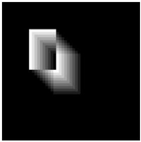
Motion is a valuable tool for segmenting images, as it allows us to differentiate between static and moving components within a scene. This segmentation method is especially beneficial in dynamic applications like robotics, autonomous navigation, and scene analysis, where objects of interest often move relative to the background.

The two main techniques for using motion in segmentation are spatial techniques and frequency domain techniques. Below, we will discuss each approach in detail.

Spatial Techniques

Basic Approach: Difference Images

In spatial techniques, one of the simplest ways to detect motion is to compute a difference image by comparing two frames (images) taken at different times. This technique assumes a reference image containing only stationary elements and a second image with some moving objects. When we subtract the reference image from the subsequent image, the difference image retains only the moving components, as the stationary elements cancel out.

The difference image between two frames taken at times $t_i$ and $t_j$ is defined as:

where:

• $f(x, y, t_i)$ and $f(x, y, t_j)$ are the pixel intensities at coordinates $(x, y)$ in the frames at times $t_i$ and $t_j$,
• $T$ is a threshold that defines significant intensity differences,
• $d_{ij}(x, y) = 1$ only if the intensity difference at that pixel exceeds $T$, indicating motion at that pixel.

Thus, $d_{ij}(x, y) = 1$ values are interpreted as locations of motion in dynamic image processing.

Addressing Noise

In real-world applications, noise can introduce 1-valued entries in $d_{ij}(x, y)$ due to random fluctuations, not actual motion. To address this, we use connectivity-based filtering. Specifically:

• Isolated 1-valued points are ignored, as they likely result from noise.
• Only 4- or 8-connected regions of 1-valued points that contain a minimum number of pixels are considered valid motion. This approach may ignore small or slow-moving objects, but it improves the accuracy of motion detection by reducing noise.

Accumulative Difference Images (ADI)

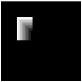
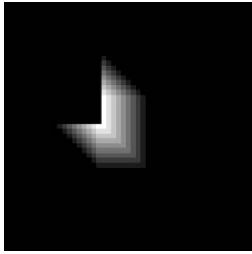
For extended analysis, an Accumulative Difference Image (ADI) can be used to track motion across a sequence of frames. The ADI compares a reference frame to each subsequent frame, incrementing a counter at each pixel location whenever a difference above the threshold $T$ is detected. This approach helps emphasize regions with consistent movement over time.

Three types of ADIs are commonly used:

1. Absolute ADI: Tracks any intensity difference.
2. Positive ADI: Tracks only positive intensity differences, assuming moving objects have higher intensities.
3. Negative ADI: Tracks only negative intensity differences, assuming moving objects have lower intensities.

Each ADI type is defined recursively:

• Absolute ADI $A_k(x, y)$:

  $$A_k(x, y) = \begin{cases} A_{k-1}(x, y) + 1, & \text{if } |R(x, y) – f(x, y, k)| > T \\ A_{k-1}(x, y), & \text{otherwise} \end{cases}$$

• Positive ADI $P_k(x, y)$:

  $$P_k(x, y) = \begin{cases} P_{k-1}(x, y) + 1, & \text{if } R(x, y) – f(x, y, k) > T \\ P_{k-1}(x, y), & \text{otherwise} \end{cases}$$

• Negative ADI $N_k(x, y)$:

  $$N_k(x, y) = \begin{cases} N_{k-1}(x, y) + 1, & \text{if } R(x, y) – f(x, y, k) < -T \\ N_{k-1}(x, y), & \text{otherwise} \end{cases}$$

Here, $R(x, y)$ is the reference frame, and $f(x, y, k)$ is the intensity at the $k$-th frame.

Frequency Domain Techniques

In the frequency domain, motion detection involves Fourier transform analysis of a sequence of image frames. Suppose we have a sequence of frames generated by a stationary camera, capturing an object moving at a constant velocity on a homogeneous zero-intensity background.

1. Fourier Transform of the Sequence: A single moving object’s movement between frames will produce a sinusoidal pattern in the Fourier domain, with the frequency of this sinusoid corresponding to the object’s velocity.

2. Example Analysis: Suppose the object is at position $(x_0, y_0)$ in the first frame. If the object moves by one pixel per frame along the x-axis, then the 1D projection along the x-axis for frame $t$ yields a term proportional to $\exp(j 2 \pi a_1 (x_0 + t) \Delta t)$, where $a_1$ is a spatial frequency component, and $\Delta t$ is the time interval between frames.

   By applying a Fourier transform, this leads to a complex sinusoid with frequency related to the object’s velocity:

   $$u_1 = a_1 V_1$$

   where $u_1$ is the frequency in the Fourier domain, and $V_1$ is the velocity in pixels per frame in the x-direction.

3. Velocity Components: A peak search in the Fourier transform reveals the frequency components. Dividing this frequency by the scaling factor $a_1$ gives the velocity component along the x-axis. A similar process provides the velocity component in the y-axis.

4. Interpretation of Static and Moving Elements: In sequences with static backgrounds, the Fourier transform produces a peak at zero frequency (dc component). Moving objects create additional peaks at frequencies proportional to their velocities, making it possible to differentiate between static and dynamic elements.

References

- Thresholding and Region-Based Methods
- Otsu, N. (1979). “A Threshold Selection Method from Gray-Level Histograms.” IEEE Transactions on Systems, Man, and Cybernetics, 9(1), 62–66. This paper introduces Otsu’s method, which is widely used for automatic thresholding.
- Gonzalez, R. C., & Woods, R. E. (2018). Digital Image Processing (4th ed.). Pearson.
- Clustering-Based Methods
- MacQueen, J. B. (1967). “Some Methods for Classification and Analysis of Multivariate Observations.” Proceedings of the Fifth Berkeley Symposium on Mathematical Statistics and Probability, 1, 281–297.
- Jain, A. K., Murty, M. N., & Flynn, P. J. (1999). “Data Clustering: A Review.” ACM Computing Surveys (CSUR), 31(3), 264–323.
- Edge Detection and Active Contours
- Canny, J. (1986). “A Computational Approach to Edge Detection.” IEEE Transactions on Pattern Analysis and Machine Intelligence, 8(6), 679–698.
- Kass, M., Witkin, A., & Terzopoulos, D. (1988). “Snakes: Active Contour Models.” International Journal of Computer Vision, 1(4), 321–331.
- Fourier Transform and Frequency Domain Segmentation
- Pratt, W. K. (2007). Digital Image Processing: PIKS Inside (4th ed.). Wiley.
- Deep Learning for Segmentation
- Ronneberger, O., Fischer, P., & Brox, T. (2015). “U-Net: Convolutional Networks for Biomedical Image Segmentation.” In International Conference on Medical Image Computing and Computer-Assisted Intervention (pp. 234–241). Springer.
- Long, J., Shelhamer, E., & Darrell, T. (2015). “Fully Convolutional Networks for Semantic Segmentation.” Proceedings of the IEEE Conference on Computer Vision and Pattern Recognition (pp. 3431–3440).
- Comprehensive Resources on Image Segmentation
- Szeliski, R. (2010). Computer Vision: Algorithms and Applications. Springer. This textbook provides a deep dive into various segmentation methods and their applications in computer vision.
- Zhang, Y. J. (1996). “A Survey on Evaluation Methods for Image Segmentation.” Pattern Recognition, 29(8), 1335–1346.
- Further Reading and Tutorials
- MathWorks Documentation: “Image Segmentation Techniques.”
- OpenCV Documentation: “Image Segmentation.”