Subband coding is a signal processing technique primarily used in digital audio, speech, and image compression. The main idea behind subband coding is to split a signal into different frequency components, called subbands, and then process each subband independently. By compressing these subbands separately, we can achieve more efficient data representation and compression.
This method is widely used in applications like audio codecs (MP3, AAC), image compression (JPEG 2000), and video compression (MPEG standards).
Key Concepts in Subband Coding
To fully understand subband coding, let’s dive into the mathematical and conceptual components involved.
1. Decomposition of the Signal
The first step in subband coding is decomposing the signal into different frequency subbands. This is typically done using filters—specifically, bandpass filters. These filters separate the signal into components that represent different parts of the frequency spectrum.
Let’s assume the input signal is a discrete-time signal . The goal is to decompose this signal into multiple subbands. Each subband represents a different frequency range, and we process each one separately.
Mathematically, we apply a filter bank to the signal. A filter bank consists of several filters that divide the signal into different frequency bands. Suppose we want to decompose the signal into two subbands: a low-frequency subband and a high-frequency subband .
This can be written as:
Where:
- is a low-pass filter.
- is a high-pass filter.
- represents convolution.
2. Downsampling
Once the signal is filtered into subbands, we can reduce the sampling rate of each subband without losing important information. This is because each subband now contains a limited range of frequencies, so we can represent it using fewer samples.
The process of reducing the sampling rate is called downsampling. For instance, if the original signal was sampled at a rate , we can downsample each subband by a factor of 2 (or higher). This reduces the data size significantly, which is crucial for compression.
Mathematically, downsampling by a factor of 2 can be written as:
This step effectively halves the number of samples in each subband, reducing the overall data size.
3. Quantization
After downsampling, each subband is quantized to reduce the precision of the signal values. Quantization is a crucial step in data compression as it allows the signal to be represented using fewer bits. The trade-off is that quantization introduces some distortion into the signal, but careful design can minimize the impact.
Quantization can be uniform or non-uniform. In uniform quantization, the signal values are mapped to fixed intervals, while in non-uniform quantization, the intervals may vary based on the signal characteristics.
For example, let’s assume that the downsampled subband takes continuous values between 0 and 1. In a 4-bit uniform quantization scheme, each value is mapped to one of 16 possible levels. The quantized version of the signal, , would have values restricted to these levels.
Mathematically, this can be expressed as:
Where represents the quantization function.
4. Encoding
Once quantization is completed, the subbands are encoded using an entropy coding technique like Huffman coding or arithmetic coding. This step is crucial for achieving high compression ratios. The encoding process takes advantage of the fact that some signal values or patterns occur more frequently than others and assigns shorter codes to frequent patterns and longer codes to infrequent ones.
5. Reconstruction (Decoding)
To reconstruct the original signal, the inverse operations of the encoding process are applied. The process of reconstruction involves:
- Decoding the quantized and encoded data.
- Upsampling each subband to the original sampling rate.
- Filtering each subband using the corresponding reconstruction filters.
- Summing the filtered subbands to reconstruct the original signal.
Mathematically, the reconstruction of the original signal from the low-pass and high-pass subbands and (upsampled versions) is given by:
Where the subbands are first upsampled and then passed through corresponding reconstruction filters, and , which are complementary to the analysis filters and .
Example: Simple Subband Coding of a Signal
Let’s illustrate the subband coding process with a simple example.
Step 1: Signal Decomposition
Consider a discrete-time signal that consists of both low and high-frequency components. We apply a two-channel filter bank to decompose the signal into a low-frequency subband and a high-frequency subband.
Step 2: Downsampling
We downsample both subbands by a factor of 2, reducing the number of samples in each subband by half.
Step 3: Quantization
The downsampled subbands are then quantized using a simple uniform quantizer. Let’s say we use 8 bits for the low-frequency subband and 4 bits for the high-frequency subband. This reduces the bit rate of the signal.
Step 4: Encoding
We encode the quantized subbands using Huffman coding, which compresses the data based on the frequency of occurrence of each quantized value.
Step 5: Reconstruction
At the receiver, we reverse the process by decoding the Huffman codes, upsampling the subbands, filtering them, and summing them to reconstruct the original signal .
Mathematical Summary
Analysis filters:
Downsampling:
Quantization:
Upsampling:
Reconstruction:
Wavelets and Multiresolution Processing
In digital signal processing (DSP), wavelets and multiresolution analysis are fundamental tools used for signal decomposition and reconstruction, particularly useful in applications like image processing, compression, and data analysis.
1. Filter Banks and Their Importance
A filter bank is a set of filters that decompose a signal into multiple components, each representing a different frequency band. The primary goal of using filter banks is to separate the input signal into subbands—low and high frequency components—that can be processed independently and then recombined.
1.1 Two-Band Filter Bank
Consider a two-band filter bank consisting of two filters:
- (low-pass filter)
- (high-pass filter)
These filters split the input signal into two frequency bands: low and high frequency. The analysis filter bank decomposes the signal, and the synthesis filter bank is used to reconstruct the signal.
The input signal is divided as follows:
- The low-pass filter captures the low-frequency components of the signal.
- The high-pass filter captures the high-frequency components.
After decomposition, the signal can be processed and later combined in the synthesis filter bank to reconstruct the original signal, represented as:
where and represent the filtered subbands.
1.2 Modulated Filters
The filters can also be modulated versions of each other, meaning they have alternating signs in their coefficients. For example, if is a reflection or order-reversed version of , it can be modulated as:
This property is important in perfect reconstruction, where the analysis and synthesis filters are carefully designed to guarantee no loss of information during signal processing.

2. Subband Coding
Subband coding is a technique used to compress signals by breaking them into subbands, encoding the subbands independently, and then reconstructing the original signal with minimal error. This is especially useful in audio and image compression, where different frequency bands contain different levels of detail.
In subband coding, the input signal is passed through a bank of filters, typically designed to divide the signal into low and high frequency components. These components are easier to compress, as they often contain redundant or irrelevant information for the reconstruction.
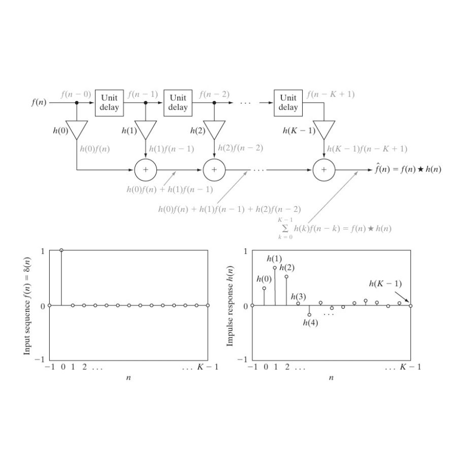
For instance, in Figure 7.4, the process of subband coding is illustrated where the input sequence is delayed through a series of unit delays and then filtered using convolution. The delayed sequence is represented as:
The output of this system, after passing through the delays and filters, is computed using convolution, defined as:
where denotes convolution, and the result is a sum of delayed versions of the input signal, multiplied by filter coefficients.
3. Mathematical Concepts in Filter Banks
Several key mathematical formulas describe the operations within filter banks. Let’s discuss some important equations shown in the figures.
3.1 Order-Reversed Filters
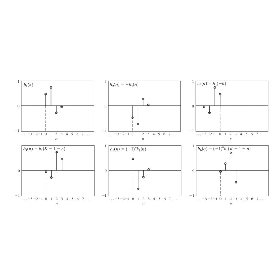
Two filters, and , are order-reversed versions of the filter . They are defined as:
These filters reflect or shift the original filter about the vertical axis. When order-reversed, their responses remain identical, but the relationship between the two filters becomes clearer in signal processing applications.
3.2 Modulated Version of a Filter
Modulation changes the sign of coefficients depending on whether is odd or even. A modulated version of the filter , denoted , is:
This modulation is essential for generating high-pass filters from low-pass filters, which helps in creating orthogonal filter banks.
3.3 Perfect Reconstruction Condition
In filter banks, the goal is to achieve perfect reconstruction—where the signal is decomposed and then reconstructed without any loss. The impulse responses of the analysis and synthesis filters must meet certain conditions for this to be possible.
One such condition is the biorthogonality condition, which ensures that the filter coefficients are properly aligned. It is defined as:
where represents the Kronecker delta function. This condition guarantees that the original signal can be perfectly recovered from its subbands.

4. Example: Filter Coefficients and Impulse Response
Let’s take an example where the input to the filter is a unit discrete impulse, denoted . The impulse response of the filter , which characterizes the filter, is the output when the input is an impulse.
If the input is , the output of the filter is simply the filter coefficients:
For instance, a filter with coefficients will output the same sequence when an impulse is passed through it.
In Figure 7.5, six different impulse responses are shown, demonstrating how a signal is transformed by various filters, including:
- Sign-reversed filters
- Order-reversed filters
- Modulated filters
5. Conclusion
In summary, wavelets and multiresolution processing are powerful techniques in digital signal processing. The use of filter banks and subband coding allows signals to be broken down into different frequency components, manipulated, and perfectly reconstructed. The mathematical tools, such as modulated filters, order-reversed filters, and the biorthogonality condition, ensure that the filters perform effectively, leading to successful applications in data compression, image processing, and beyond.
By understanding the fundamental principles of wavelets and filter banks, signal processing becomes a powerful framework for efficiently handling a wide range of applications, from telecommunications to multimedia systems.
Applications of Subband Coding
Audio Compression: Subband coding is the foundation of many audio compression algorithms like MP3 and AAC. The audio signal is split into different frequency bands, and each band is compressed based on the auditory system’s sensitivity to different frequencies.
Image Compression: In JPEG 2000, an image is split into multiple frequency subbands, and each subband is compressed separately, leading to efficient compression with minimal quality loss.
Speech Coding: Subband coding is also used in speech coding, where it helps in reducing the bit rate while maintaining intelligibility and clarity of speech.
References
- Vetterli, M., & Kovacevic, J. (1995). Wavelets and Subband Coding. Prentice Hall.
- Said, A., & Pearlman, W. A. (1996). A new, fast, and efficient image codec based on set partitioning in hierarchical trees. IEEE Transactions on Circuits and Systems for Video Technology, 6(3), 243-250.
- Gersho, A., & Gray, R. M. (1992). Vector Quantization and Signal Compression. Springer Science & Business Media.
- Noll, P. (1993). MPEG digital audio coding. IEEE Signal Processing Magazine, 10(3), 59-81.
Discusses the use of subband coding in the MPEG audio coding standards and its role in achieving compression for digital audio. - Jayant, N. S., & Noll, P. (1984). Digital Coding of Waveforms: Principles and Applications to Speech and Video. Prentice-Hall.
- Bosi, M., & Goldberg, R. E. (2003). Introduction to Digital Audio Coding and Standards. Springer.
- Strang, G., & Nguyen, T. (1996). Wavelets and Filter Banks. Wellesley-Cambridge Press.
